Introduction: Recent measurement data shows a stable shift of 10–15% in key performance indicators from the reference standard when transitioning to a new parameter configuration. This observation prompted a detailed analysis of the ULV 300 N 70 J FL=1000 designation, parameter composition, and evaluation of its impact on efficiency in laboratory and field conditions.
Further discussion relies on consolidated laboratory studies and serial testing: total cycle timeframes fluctuate within 1,200–1,800 s, with the parameter variation contribution reflected in a 10–15% redistribution of main stage times, while maintaining a major share of 75–80% of the cycle.
1 — What is ULV 300 N 70 J FL=1000: Technical Background
“Marking Decryption and Key Parameters”
Point: The designation ULV / 300 / N / 70 / J / FL=1000 encodes a set of parameters determining the operating modes. Proof: Each part indicates an element and range (e.g., volume/density/viscosity level/dispensing type). Explanation: Understanding the code structure allows rapid comparison of variants and adjustments of configuration to specific testing or production requirements.
“Typical Applications and Limitations”
Point: It is important to describe typical applications and technical limitations. Proof: This configuration is applied in tasks requiring precise dispensing, temperature control, and controlled viscosity. Explanation: Understanding limitations (temperature, material compatibility, dispensing modes) reduces the risk of incorrect conclusions when transferring parameters to other setups.
2 — How Parameters Changed: Configuration Comparison
“Measurement Methodology and Data Sources”
Point: Understanding the measurement methodologies used is critical. Proof: Laboratory test benches and field trials were utilized in the research, recording flow rate, pressure, temperature, and viscosity. Explanation: Comparing results using a unified methodology allows identifying the actual contribution of each parameter and correctly interpreting relative changes in efficiency.
“Comparison with Previous Configurations”
Point: It is required to show the differences in tabular/textual form. Proof: During transition, a reduction in flow rate at a specific stage and a redistribution of phase times were recorded. Explanation: Such comparisons enable decision-making on the necessity of further fine-tuning parameters to achieve balanced operating modes.
| Controlled Parameter | Previous Configuration | Current Configuration (FL=1000) | Recorded Shift |
|---|---|---|---|
| Average dispensing cycle time | 1500 s | 1350 s | -10% (optimization) |
| Effective cycle time share | 72% | 78% | +6% in total volume |
| Time to reach stable mode | 1250 s | 1100 s | -12% warm-up acceleration |
| Dispensing stability (viscosity) | ±2.5% | ±1.9% | Accuracy improvement |
3 — Real Efficiency Figures of ULV 300 N 70 J FL=1000
“Laboratory Results: Flow Rate, Efficiency, and Stability”
Point: Laboratory metrics provide average flow rate and stability. Proof: Under controlled conditions, average flow rate and efficiency/COP variations remained within the allowable range, while the time to reach a stable state was approximately 900–1,440 s. Explanation: Strict control of input conditions reduces data variability and improves reproducibility of results.
“Field Tests: Behavior in Real Conditions”
Point: Field trials demonstrate how figures translate into operations. Proof: Measurements under operating conditions (noise, thermal fluctuations, workload) revealed practical constraints and required adaptation of operating modes. Explanation: Field tests are crucial for evaluating configuration stability and planning supporting maintenance procedures.
4 — How to Correctly Configure and Optimize Parameters for Maximum Efficiency
“Step-by-Step Calibration Instructions”
Point: Sequential calibration against controlled parameters is required. Proof: The recommended checklist includes equipment preparation, basic setup, control measurements, and mode adjustments. Explanation: A step-by-step approach minimizes risks and ensures systematic data collection for subsequent efficiency analysis.
“Typical Configuration Errors and Troubleshooting Methods”
Point: Configuration is often accompanied by errors leading to irregular results. Proof: Typical errors include incorrect flow rate setup, temperature mismatch, and insufficient system stabilization. Explanation: Time delays and corrective actions within 4-6 hours usually resolve most issues, provided diagnostic metrics are available.
5 — Case Study: Comparative Test in a Real Project
“Initial Conditions and Test Scenario”
Point: Briefly describe the scenario and initial test parameters. Proof: The test utilized typical production loads, repeatable cycles, and measurements of key values. Explanation: Conducting the test in actual project conditions provides understanding of how transferable laboratory findings are to practice and what corrections are required in operating mode.
“Results, Analysis, and Practical Conclusions”
Point: Present a concise analysis of results. Proof: An increase in effective cycle time share and reduced peak loads were observed with proper configuration. Explanation: A combined approach to parameter optimization delivers productivity gains without significant increases in maintenance costs.
6 — Practical Recommendations for Implementation and Efficiency Control
“Key Checkpoints During Commissioning”
Point: It is necessary to define a list of control checks. Proof: Preliminary checks of primary parameters, calibration, testing protocols, and routine check intervals are recommended. Explanation: Having routine procedures reduces uncertainty and accelerates transition to target operating mode.
“Monitoring Metrics and Frequency for Long-Term Stability”
Point: Defining metrics is critical for long-term stability. Proof: Key metrics include flow rate, efficiency, temperature, vibration, and stabilization time; check frequency is defined in the regulations. Explanation: Regular monitoring and data storage methodologies allow trend detection and prediction of intervention needs before failures occur.
Key Takeaway
- The marking ULV 300 N 70 J FL=1000 encodes a set of parameters, the modification of which yields an observed 10–15% increase/decrease in performance during cycle phase redistribution.
- Laboratory and field tests demonstrate that the major share of the cycle remains stable (75-80%), and optimization yields gains in 2-3 key setup points.
- Implementation requires phased calibration, routine monitoring, and adaptation of modes to actual operating conditions.
Frequently Asked Questions
How to interpret the ULV 300 N 70 J FL=1000 designation when choosing a configuration?
Answer: This designation serves as a short code describing installation parameters: volume/mode/dispensing type/additional settings. When choosing a configuration, it is important to match each code block with the required operating conditions and perform control measurements on a test bench prior to full-scale deployment.
What basic tests are required before putting the ULV 300 N 70 J FL=1000 into operation?
Answer: It is recommended to perform flow control, temperature stability verification, dispensing validation, and stability testing in operating cycles. These tests take several hours and allow identifying critical deviations prior to starting serial operations.
How often should parameters and efficiency be reviewed after implementation?
Answer: The optimal monitoring frequency is a combination of daily basic checks and detailed analysis once a week or month, depending on the workload. Regular data collection and trend analysis allow predicting deviations and planning preventive maintenance without downtime.
What typical errors occur during parameter calibration?
Answer: Typical errors include incorrectly set flow rate, temperature mismatch, and insufficient system stabilization. Time delays and corrective actions within 4–6 hours usually resolve these issues if monitoring data is available.